Notes on Hiroki Tanioka's Introduction to Deep Learning
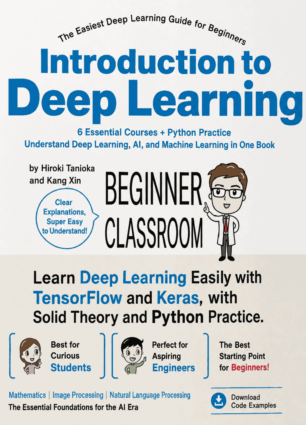
Introduction to Deep Learning by Hiroki Tanioka and Kang Xin
Original notes here.
Read until the end to get a bonus. Enjoy reading.
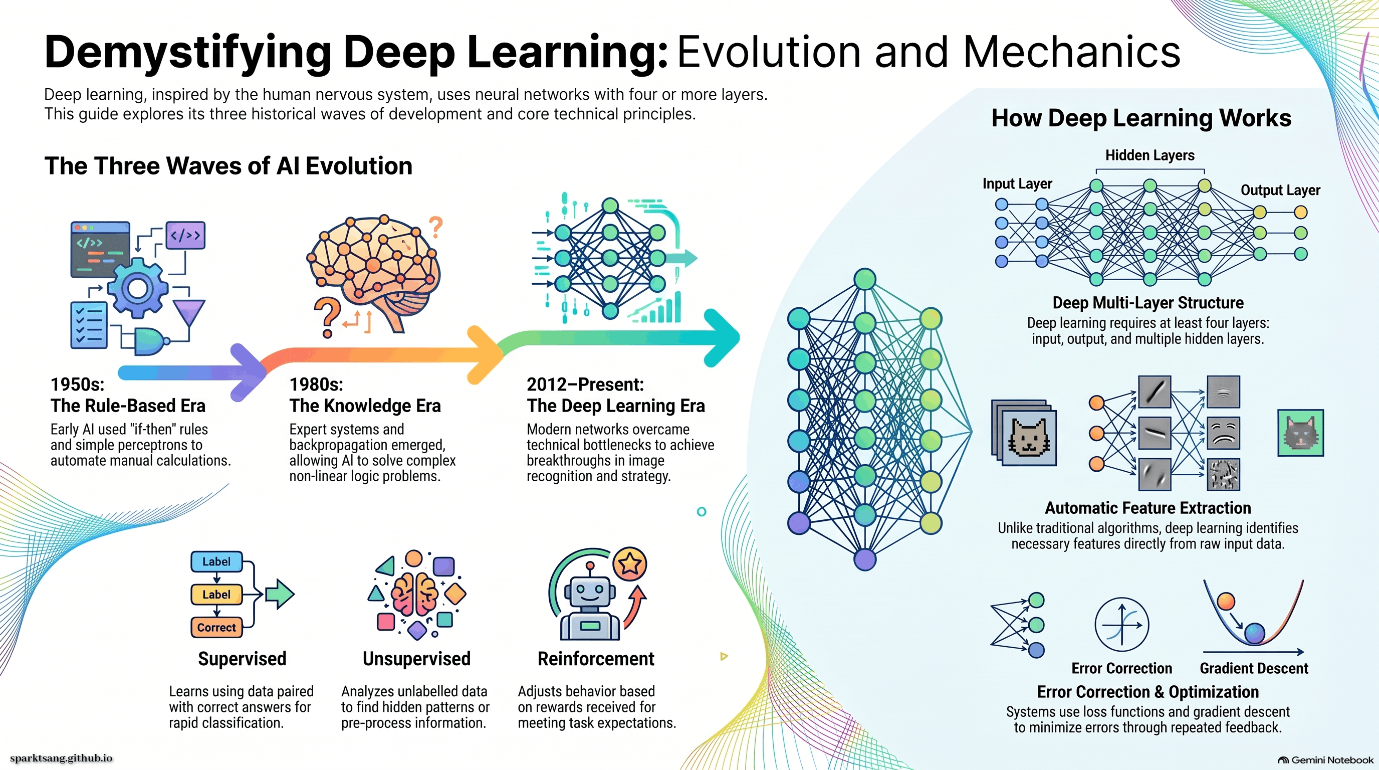
“Deep Learning,” also known as “deep neural networks,” is created by making “neural networks” (modeled on the human nervous system) deeper.
In other words, they are multi-layer neural networks, with at least four layers—more than the three-layer structure consisting of one input layer, one hidden layer, and one output layer. There are multiple hidden layers.
“Neural network” is one type of algorithm in the field of “machine learning.”
The first wave of artificial intelligence in the 1950s replaced manual calculation with the automatic execution of rules, leading to research into rule bases and the development of many automata.
Rule base: an “if A, then B” algorithm library; automaton: a program in which the input is x and the output is y, which can adjust itself according to its internal state h, i.e. f(x, h). Applications included kana-to-kanji conversion and vending machines.
In 1958, Frank Rosenblatt published the perceptron, which became the foundation of neural networks. It imitated the structure of biological neurons in an attempt to create intelligence capable of handling complex problems.
The original perceptron had only one layer, followed by models with two layers for input and output, and then three layers with the addition of a hidden layer.
The boom gradually faded after Marvin Minsky demonstrated that a simple perceptron could not solve the exclusive-or (XOR) problem.
The second wave of artificial intelligence in the 1980s developed large knowledge bases that collected human experience, knowledge, and common sense in an attempt to achieve artificial intelligence closer to human intelligence—knowledge-based AI.
Specialized knowledge bases designed for specific fields were also common; these were known as expert systems, such as Deep Blue.
In 1967, Shunichi Amari demonstrated a usable backpropagation algorithm. Finally, in 1986, David E. Rumelhart, Geoffrey E. Hinton, and others showed that it was effective, establishing that the exclusive-or logic problem, which a simple perceptron could not handle, could in fact be solved.
The boom gradually faded because increasing the number of layers led to declining performance, the vanishing gradient problem, and the problem of getting stuck in local minima.
In the 1990s, Hinton and others developed methods showing that even neural networks with four or more layers could overcome the vanishing gradient and local optimization problems. In 2012, his team used deep neural networks to achieve image-recognition accuracy far ahead of the competition, bringing deep learning into the spotlight and triggering the third wave of artificial intelligence.
Deep learning has also been applied to automatic image generation, natural language generation, machine translation, robot control, and so on. In 2016, AlphaGo defeated the world’s top Go players.
Machine learning is divided into:
Supervised learning: learning by being given data together with the correct answers.
In addition to neural networks, this includes Naive Bayesian classifiers, logistic regression, decision trees, and support vector machines.
These methods allow computers to perform classification rapidly and accurately.
Unsupervised learning: no correct answers are provided; the system learns only from the data.
This includes algorithms in fields such as k-means, cluster analysis, and dimensionality reduction, as well as autoencoder techniques in neural networks. These are analytical methods that make unseen data easier to understand, or are used as pre-processing for supervised learning.
Reinforcement learning: rather than directly indicating the answer, the system is given a reward based on whether the outcome of a task meets expectations, allowing it to adjust itself.
This includes Q-learning, the SARSA method, and the Monte Carlo method.
Machine learning cannot directly read and learn from raw data. Pre-processing converts raw data into a data format that machine-learning programs can read.
Conventional machine-learning algorithms generally need to extract the necessary features for learning from the input data. One reason deep learning has attracted so much attention is that it can already achieve good performance without going through a separate “feature extraction” stage.
Input data for learning can be divided into batch learning and online learning. The former integrates multiple input data points and learns from them collectively, determining whether the overall judgment is correct; online learning provides feedback one item at a time.
Machine-learning performance is evaluated in terms of training time, inference time, and overall accuracy/loss.
Standards for inference accuracy include accuracy and loss. There are also recall, precision, false positives, false negatives, and so on.
Extremely high accuracy on specific training data does not necessarily extend to unseen data. This phenomenon is called overfitting. The ability to handle unseen data is called generalization ability.
A neuron is the basic unit of the human brain. In terms of an artificial neural network, it can be represented by the following equation:
\(z = f(\mu) = f\left(\sum_{i=1}^{n} (w_i x_i - h)\right); i, j\)
x = input value; w = weight coefficient; h = threshold
The simplest model is: z = 1 if μ > h else 0
This is a step function, which looks like a staircase when plotted.
The mechanism for learning through an artificial neural-network model is called the perceptron. It is known to be equivalent to logistic regression in the field of statistics, which was also published in 1958. This coincidence is quite interesting and also made a major contribution.
A function that outputs 1 when a certain condition is met and 0 otherwise is called an activation function. There are various kinds, including:
S function / Sigmoid function: \(f(\mu) = \frac{1}{1 + e^{-\mu}}\)
ReLU function: h(x) = x if x > 0 else 0
There are two rules for learning how to modify the weights used in combinations: the Hebbian Rule and the Delta Rule.
Hebbian Rule: \(\Delta w_{ij} = \lambda x_j y_i$; $\Delta w_{ij}\) = change in weight
Since y can only be 0 or 1, this can be expressed as:
Δw = λx if y triggered else 0
Delta Rule: the larger the difference between the answer and the output, the larger the weight adjustment; at the same time, the larger the input value, the larger the adjustment.
\(w(t+1) = w(t) + \eta \delta x(t); \quad \delta = y'(t) - y(t)\)
The contents in parentheses are written as subscripts to the variables.
When the output answer is correct:
\(f(w) = \lim_{n \to \infty} \frac{1}{n} \sum_{i=1}^{\infty} \left(y'(i) - y(i)\right)^2\)
The above approach minimizes the function f(w), gradually correcting it through repeated attempts.
Linearly separable problems can be judged relatively easily. The XOR problem is a representative example of a non-linearly separable problem.
David E. Rumelhart proposed making the perceptron hierarchical: first use OR and NAND, then apply AND to the two results to produce NAND, thereby solving the non-linearly separable problem.
Taking supervised learning as an example, the steps are as follows: prepare the data, distinguish the input from the correct answers, feed the input into the neural network and have it classify the data, provide feedback on the differences, and update the parameters.
The function used to measure error is called the loss function. Common forms include mean squared error and cross-entropy loss.
Mean squared error: \(E = \frac{1}{2} \sum_{k} (y(k) - t(k))^2\)
The 1/2 is included to cancel out the constant 2 that appears after differentiation.
Cross-entropy: \(E = - \sum_{k} \left(t(k) \log_e(y(k))\right)\)
This can be used in situations where the difference cannot simply be calculated, such as distinguishing cats from dogs.
y is the machine’s prediction; t is the correct answer.
With a finite amount of data, one could simply change the values at random and search for the method that produces the smallest error. But once the combinations become enormous, this approach becomes impractical.
Gradient descent can solve this problem. It is like trying to find the highest mountain in the world: first climb a nearby peak, look for a higher mountain, and repeat the process.
For example, with \(y = x ^ 2\), the minimum is at the point where the derivative is 0. The gradient method compares the derivative values and searches in the downward direction. The size of the steps also needs to be appropriate, and this can be determined by the learning coefficient η. Because this is not a parameter directly related to the model itself, it is called a “hyperparameter.”
There are various gradient descent optimization algorithms, including the steepest descent method, Newton’s method, and Stochastic Gradient Descent.
Backpropagation is one of the most effective learning methods for multi-layer neural networks. One of its key mathematical principles is the chain rule:
\(\frac{\partial y}{\partial x} = \left(\frac{\partial y}{\partial z}\right) \times \left(\frac{\partial z}{\partial x}\right) \approx \left(\frac{\Delta y}{\Delta z}\right) \times \left(\frac{\Delta z}{\Delta x}\right)\)
In the example of a character-recognition program, Sequential() is used to select the basic model.
Dense defines the first layer, while Activation sets the activation function; here, ReLU is used.
Dropout randomly resets some inputs to 0 to prevent overfitting. 0.2 means that 20% of the inputs will be reset.
Finally, the output Activation uses softmax to determine, based on probability, which output result is most likely.
The Param count for Dense 1 is (784+1)×512. Each layer has one additional parameter because Bias has been added to replace the threshold. The second layer is (512+1)×512, and the last is (512+1×10).
model.compile compiles the prepared learning model, converting it into a form that the machine can process.
loss is specified as categorical_crossentropy, using cross-entropy as the loss criterion. Early stopping is a function that allows learning to end early once a certain level has been reached.
training.log outputs a record of the learning process; model.fit progressively updates the model parameters.
After repeatedly learning from the training data, the loss gradually decreases. But with the test data, repeated learning does not lead to much of a decrease (comparing loss with val_loss), indicating overfitting.
Curse of dimensionality: the learning effect may not necessarily be good with too few neurons, and repeated learning may also result in overfitting. But with a complex network, the number of possible parameter combinations can also explode.
A convolutional neural network is an important core technology in deep neural networks, designed for computer-vision tasks.
Convolution means focusing on a small region at a time and learning the entire input image by moving this focus across it.
The most common movement is from left to right and from top to bottom, called sliding.
If the input is a 6×6 square and the receptive field is 3×3, the output is 4×4, i.e. W-F+1.
Artificial-intelligence research includes both top-down and bottom-up approaches: the former attempts to achieve intelligence from the theoretical perspectives of mathematics and computer science, while the latter imitates the structure of neurons in the brain.
Child-development and developmental psychologist Alison Gopnik explains that human children’s methods of learning can also broadly be divided into two types: top-down learning, which makes inferences based on existing knowledge, and bottom-up learning, which learns from actual phenomena.
Although deep learning emerged from top-down research, the learning mechanism itself is bottom-up.
Example programs from this book can be found at: www.sotechsha.co.jp/sp/1187
Read through page 152. The remaining content concerns image recognition and natural language processing.
Last updated: August 27, 2020
Thank you for reading until the end. This is a bonus infographic just for you.